
Numbers Far Afield
Published by Reblogs - Credits in Posts,

Numbers Far Afield
"To learn all that is learnable;
(Vejur, née Voyager 6, in Star Trek: The Motion Picture)
to deliver all collected data
to the Creator on the third planet.
That is the programming."
Imagine a vast growing sphere centered on the Earth with a radius of fifteen billion miles, the distance a beam of light travels in a day. This is the anthroposphere: the patch of the universe into which humanity and its artifacts have spread. At its periphery – indeed, defining its periphery – is a one-ton device hurtling away from us at forty-thousand miles per hour while sending radio signals toward Earth with a broadcast power of twenty watts. That’s only a tiny fraction of the wattage used by commercial radio stations on Earth, yet somehow Voyager 1, with its puny transmitter, is still executing its mission of gathering data about our solar system and relaying that data back to far-off Earth. And part of the technology that makes this feat possible is an algebraic construct that nobody even dreamed of two centuries ago: the arithmetic of finite fields.

Actually, I shouldn’t be so confident that nobody back then dreamed of finite fields; Carl Friedrich Gauss (1777–1855) may have. He was known for not writing up his ideas until they had matured sufficiently, which in some cases meant never writing them up at all.
In his Disquisitiones Arithmeticae, published in 1801, Gauss introduced the idea of two integers being congruent to one another relative to some third integer that he called the modulus. (If you need a refresher on modular arithmetic, or if it’s new to you, check out my essay The Triumphs of Sisyphus.) Just over thirty years later, in an 1832 monograph, he introduced number systems that contain not just the integers but also some extra numbers thrown in, such as the Gaussian integers, that is, all numbers of the form a + bi where i is the square root of −1. Gauss might have wondered what form modular arithmetic would take in other number systems like these. If he did pursue this, he never reached conclusions that he thought were worth publishing.1 But let’s see what kind of modular arithmetic we get when we impose the modulus 2 on the Gaussian integers and on another similar number system, doing the same sort of lumping-together we did when we looked at the integers modulo m.
IN SEARCH OF RECIPROCATION
To gear up, let’s remind ourselves how modular arithmetic works when we impose the modulus 4 on the ordinary integers. In mod 4 arithmetic, we treat two numbers as being the same – or, in technical language, congruent – if they differ by a multiple of 4, so for example 2 times 2 is 0. Here’s (part of) a number line for the integers in which every integer is replaced by the remainder it leaves when you divide it by 4.

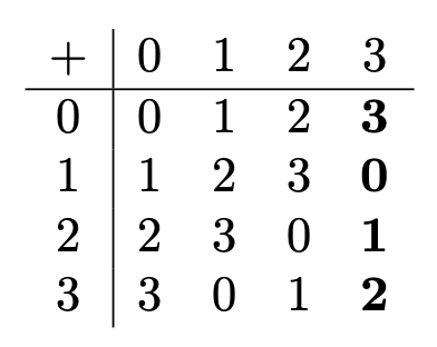
Here are the operation tables for addition and multiplication mod 4:

For instance, to use the first table to compute 2+3 in mod 4 arithmetic, find the place where the row marked "2" and the column marked "3" cross; since the entry there is a 1, we have 2 + 3 equal to 1 in mod 4 arithmetic, though we often use the symbol ≡ rather than the equals sign, with the modulus 4 lurking invisibly behind the "≡".
In this number system, subtraction works fine2 but division is a problem. If the trouble with division were just the usual caveat "You can’t divide by 0" it wouldn’t be so bad, but in this number system you also can’t divide by 2: the un-multiplication problem "Find x so that x × 2 is 1 mod 4" has no solution in the integers mod 4. That is, 2 has no reciprocal in this number system.
Another four-element number system with a similar defect is the Gaussian integers mod 2, consisting of 0, 1, i, and 1+i (which I’ll call j for short). Here’s a picture of the Gaussian integers in which every Gaussian integer has been replaced by the remainder it leaves when you divide it by 2.

I give more details in the Endnotes but here I’ll just say that 1+i has no reciprocal in this number system.3
We get something nicer if instead of the Gaussian integers we use the Eisenstein integers. The Eisenstein integers are the complex numbers of the form a+bγ where a and b are ordinary integers and γ (that’s what gamma looks like in WordPress, apparently) is the complex number −1/2 + i sqrt(3)/2. Don’t let those fractions and that square root scare you; all you really need to know about γ is that is satisfies the equation γ2+γ+1 = 0, or equivalently, γ2 = −γ−1. When we mod out by 2, we’re only paying attention to the parity (that is, oddness or evenness) of a and b, so we might as well restrict a and b to be 0 or 1, so that the elements of our reduced arithmetic are 0, 1, γ, and 1+γ; I’ll abbreviate the last of these as δ. Here’s a picture of the Eisenstein integers in which every Eisenstein integer has been replaced by the remainder it leaves when you divide it by 2.

And here are the operation tables for addition and multiplication of Eisenstein integers mod 2:

I won’t explain all the entries, but I’ll explain two of them. To see why γ times γ is δ, recall that in the Eisenstein integers not modded out by 2, γ times γ is −1−γ. But since −1 and +1 are the same mod 2, we can rewrite this as 1+γ, i.e. δ. Likewise, to see why δ times δ is γ, apply the distributive law to expand 1+γ times 1+γ as 1+2γ+γ2. Since γ2 = −1−γ, 1+2γ+γ2 becomes 1+2γ−1−γ, which is just γ.
In this number system, every nonzero element has a reciprocal that also belongs to the number system; specifically, 1 is its own reciprocal and γ and δ are reciprocals of each other. Consequently, division works just fine, where we perform division using the rule "To divide by an element, just multiply by its reciprocal."
The long-deferred moment has arrived when I need to bring the word "field" into the conversation. Fields are number systems in which all four of the fundamental operations of arithmetic – addition, subtraction, multiplication, and division – work nicely, at least as long as you don’t divide by the additive identity element 0.
Whenever p is prime, the integers mod p form a tidy finite field called p. But these aren’t the only finite fields; for instance, we just met a field with 4 elements, namely the Eisenstein integers mod 2. Similarly, if you take the Gaussian integers mod 3, you can construct a finite field with 9 elements.4 The full story is that whenever the number n is a power of a prime, say n = pk with p prime and k ≥ 1, then there’s a finite field5 with n elements, written as pk. One way to construct finite fields follows the approach we took with 4: start with a suitable system of algebraic numbers and mod out by a suitable prime p. But this is not how finite fields were actually invented.
A RADICAL MATHEMATICIAN
Finite fields are the creation of the revolutionary mathematician Évariste Galois (1811–1832), who died before his twenty-first birthday. He wasn’t just a mathematical revolutionary; he was also a political revolutionary who ardently supported Republican ideals in the years leading up to the French Revolution of 1830. Political embroilments, unreciprocated affection, and/or suicidal depression led him to enter into a fatal duel (see Why was Évariste Galois killed?). I’ve complained about the algebra duels of mid-millennial Italy and the adverse effect they had on the progress of mathematics, but at least in those duels, the loser lost only his job, not his life!
Galois was interested in the theory of equations and more specifically in a question that had preoccupied algebraists for many decades: Which algebraic equations can be solved using just the four standard operations of algebra (+, −, ×, ÷) along with radicals (square roots, cube roots, fourth roots, etc.)? His novel approach involved a sort of covert choreography in which the solutions of an equation swap places with each other while we’re not looking, and we observe how various permutations of the solutions leave some expressions invariant but change the values of other expressions, the way swapping the two roots r, s of a quadratic equation leaves the values of r+s and rs alone but causes the value of r−s to change sign. It was brilliant work that most mathematicians of his era were unprepared to assimilate, and it’s possible that Galois’ frustration with being misunderstood and unappreciated played a part in the train of events that led to his death.
Although some of Galois’ work was deemed incomprehensible by his colleagues and denied publication during his lifetime, some of it was published. In 1830 he published three articles, one entitled "On the theory of numbers"; it was this article that introduced finite fields to the world. Galois’ way of constructing them is to start with the integers mod p and adjoin a new element, in analogy with the way we built the complex numbers from the real numbers by adjoining a new element i satisfying i2 = −1. Under this approach, we don’t need complex numbers except as a source of inspiration. For instance, to build the field with 4 elements, we start with the two-element field 2 whose only elements are 0 and 1 and we introduce a new element called α (that’s an alpha in WordPress, apparently) with the property that α2 = α+1. Where does α come from? It doesn’t matter! We assume the existence of such an element and see what consequences the assumption leads to. If it leads to contradictions, well, then α doesn’t exist. But if the theory is consistent, then α exists just as much as it needs to; we can do math with α without worrying about its ontology. And, just as letting i combine with itself and ordinary real numbers through addition and multiplication gives rise to the field of complex numbers, letting α combine with itself and the elements of 2 through addition and multiplication gives rise to the field 4.
Finite fields are often called Galois fields in honor of their creator, and pk is often written as GF(pk). One doesn’t usually call the elements of finite fields "numbers", but they are certainly near-kindred. To heighten the resemblance, we could rebrand the elements as numbers. For instance, instead of calling the elements of GF(4) 0, 1, γ, and δ, we could call them 0, 1, 2, and 3. Then the addition table would look like this:

This seems like a crazy thing to do, since we’re subverting the meaning of the symbols 2 and 3 and altering the way they add. Yet there’s hidden sense to this nonsense. In 1901, the mathematician Charles Bouton, studying the game Nim (which seems to have been inspired by similar Chinese take-away games), realized that the foregoing strange way of adding natural numbers reflects the strategic behavior of Nim; in a certain tactical sense, a heap of size a alongside a heap of size b acts like a single heap of size c, provided that c is equal to a + b for this weird kind of addition. I wrote more about Nim in my essay When 1+1 Equals 0. Some people, adopting a coinage that I believe is due to John Conway, refer to Nim values as "nimbers".
To see the pattern governing that last addition table, it might help to replace 0, 1, 2, and 3 by their respective base-two representations 00, 01, 10, and 11:

Then the sum of the bit-pair a1a2 and the bit-pair b1b2 is the bit-pair c1c2 where c1 is the mod-2 sum of a1 and b1 and c2 is the mod-2 sum of a2 and b2.
If all these 0’s and 1’s are making you think of computers, that’s not an accident, because the next scene in the story of finite fields occurs in the dawn of the computer age.
THE LOST WEEKENDS OF RICHARD HAMMING
In the summer of 1946, thirty-one-year-old mathematician Richard Hamming (1915–1998) left the atomic bomb project at Los Alamos National Laboratories to take a job at Bell Laboratories, where a state-of-the-art binary computer called the Model V was the pride of the lab. The Model V contained nearly ten thousand relays, occupied a thousand square feet of floor space, weighed ten tons, and wasn’t intended for newbies like Hamming. Many questions that interested him couldn’t be solved by pure thought; he needed a computer like the Model V. But Hamming’s low status meant that the most he could hope for was weekend time on the Model V, and even then, only when no one else wanted to use the machine.
Input to the Model V used punched paper tape, which is not an especially reliable way of entering programs or data into a computer; it’s common for a mechanical tape-reader to misread a 1 (a hole in the tape) as a 0 (a part of the tape where a hole could have been but wasn’t) or vice versa. The Model V could also malfunction if a speck of dust landed on one of its internal relays. Fortunately the Model V’s designers had incorporated some error-detection capability into the system. Specifically, all data were expressed in the form of blocks of 5 bits, of which exactly 3 were 1’s: the "3-out-of-5 code". Here are the ten allowed blocks, corresponding to the ten decimal digits:
00111 01011 01101 01110 10011 10101 10110 11001 11010 11100
If the computer encountered a block that didn’t have exactly three 1’s, an alarm would sound and the machine’s operator could restart the job, hoping that this time there would be no errors …
… except that on weekends, when Hamming’s programs were being run, there was no operator. If the Model V detected an error during the weekend, it just terminated its current job and went on to the next one.
Hamming later recounted:
Two weekends in a row I came in and found that all my stuff had been dumped and nothing was done. I was really aroused and annoyed because I wanted those answers and two weekends had been lost. And so I said, "Damn it, if the machine can detect an error, why can’t it locate the position of the error and correct it?"
In 1948, Hamming came up with the error-correcting code that bears his name. Instead of using ten allowed blocks of length 5 as the 3-out-of-5 code does, Hamming’s code used sixteen allowed blocks, or codewords, of length 7:
0000000 0001111 0010110 0011001 0100101 0101010 0110011 0111100
1000011 1001100 1010101 1011010 1100110 1101001 1110000 1111111
This code had the desirable feature that if the tape reader (or a speck of dust in a relay) flipped a single 0 to a 1 in a block, or vice versa, the Model V would be able not merely to detect the presence of a corrupted bit but also to locate the corruption and correct it by re-flipping the flipped bit back to its original value.
Below you’ll see my attempt at a picture of the Hamming code, shown in red. I’ve used a modified, more symmetrical6 version of Hamming’s code in which the codewords are
1101000 0110100 0011010 0001101 1000110 0100011 1010001 0000000
1011000 0101100 0010110 0001011 1000101 1100010 0110001 1111111
I treated these 16 codewords as points in a 7-dimensional space and then projected that space into the plane. You see just 15 red dots, but in 7 dimensions there are 16 of them; the two codewords 0000000 and 1111111 correspond to the same point in the plane at the middle of the picture. In the 7-dimensional picture there are 128 dots in total, 16 red and the rest black, corresponding to the 128 possible bit-strings of length 7. Two dots of either color are joined by an edge if the corresponding bit-strings differ in just a single bit.
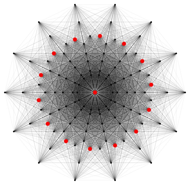
What makes this code work – that is, what makes it possible for the computer to correct all single-bit errors – is that each black dot has exactly one red neighbor; that is, each bit-string that isn’t a codeword can be turned into a codeword by flipping one bit, and this can always be done in precisely one way. It’s hard to see what’s going on in such a crowded picture, but that’s the price you pay when you squash a hyper-hyper-hyper-hypercube down into two dimensions!7
To use Hamming’s original version of his code for data transmission, you chop a long binary message into a succession of blocks of length 4. Each of the 16 possible blocks of length 4 is associated8 with a distinct codeword of length 7, and these blocks are transmitted in succession. This introduces an overhead factor of 7/4 and results in slower transmission, but what we gain is resilience in the face of channel-noise: as long as at most one bit in each transmitted codeword gets corrupted en route to its destination, the receiver can reconstruct the original message perfectly.
Hamming devised other codes of a similar kind. For instance, there’s the "extended Hamming code", obtained from the 7-bit code by appending to each codeword a bit that’s equal to the mod 2 sum of the other 7 bits.9 This 8-bit code isn’t just single-error-correcting; it’s also double-error-detecting. That is, if two bits get corrupted rather than just one, the structure of the code enables the receiver to detect the fact that two or more errors have occurred.
Over the decade that followed Hamming’s pioneering work, many people rushed in to improve on Hamming’s codes, especially in the direction of allowing more robustness in the presence of error. Why not create a code that could correct two errors in each block, or three, or more? And how low could one reduce the overhead factor?
One important thing that researchers noticed was that the Hamming code admitted a different description that used finite fields. Consider the Galois field GF(8) obtained from the 2-element field by adjoining a fictional element β satisfying the equation β3 = β + 1. Then the codewords in my symmetrical version of Hamming’s code can be described as precisely those bit-strings a1a2a3a4a5a6a7 with the property that a1β1 + a2β2 + … + a7β7 = 0 in GF(8).10
The use of finite fields helped guide researchers toward good codes, meaning codes that could correct lots of errors without incurring too much overhead. One of the best early codes based on finite fields was the BCH code of Bose, Ray-Choudhuri, and Hocquenghem.11 You know quick-response codes (aka QR codes), those square arrays of black-and-white cells that look meaningless to humans but tell a cellphone to navigate to a particular website? The black and white cells represent 0s and 1s that encode a URL using BCH codes. BCH codes are also used in CDs, DVDs, and solid-state memory devices such as flash drives.
Hamming, inspired by Eugene Wigner’s famous 1960 essay "The Unreasonable Effectiveness of Mathematics in the Natural Sciences", wrote an essay of his own in 1980 entitled "The Unreasonable Effectiveness of Mathematics". In shortening Wigner’s title, Hamming was broadening the scope of the inquiry to include for instance engineering, which strictly speaking is not a science. Hamming doesn’t mention error-correcting codes, but he could well have discussed them as an example of the way ideas developed for unworldly purposes can lend themselves to applications unimagined by their creators. Galois invented finite fields in service of the theory of equations, exploring the symmetries of algebraic expressions for their own sake. Yet somehow this purely theoretical research became foundational for the transmission and storage of data in the late twentieth century. Speaking for the mathematical community, Hamming wrote: "We have tried to make mathematics a consistent, beautiful thing, and by so doing we have had an amazing number of successful applications to the real world."
But the reverse is also true: in trying to make things work in the real world, applied mathematicians may stumble on something of timeless beauty. The extended Hamming code turned out to be relevant to the pure math problem of how one can most efficiently pack spheres in 8-dimensional space – a problem whose ultimate solution by Ukrainian mathematician Maryna Viazovska in 2016 was a major contributor toward her winning a Fields Medal in 2022. (The Fields Medal is named after Canadian mathematician John Charles Fields, no relation to Galois Fields.)
A more sophisticated code than Hamming’s (arising from GF(223)) discovered by Swiss mathematician Marcel Golay led British mathematician John Leech to discover a very dense way to pack spheres in 24-dimensional space, using spheres centered on a set of points now called the Leech lattice, which Viazovska along with others recently showed is in fact the densest way to pack spheres in 24 dimensions. In the late 20th century, the Leech lattice led to the discovery of several new kinds of symmetry, more precisely, the discovery of several new finite simple groups. Galois, who gave group theory its name, would have been pleased.
The relationship between progress in mathematics and mastery of the natural world isn’t one-way; you might even say it’s reciprocal.
RITE OF PASSAGE
If planetary civilizations have a coming-of-age ritual in which they announce their intention of becoming citizens of the cosmos, our planet’s bar mitzvah or quinceañera might be said to have taken place in the summer of 1977. That was the year we launched Voyager 1 and Voyager 2, not merely to explore our solar system and dip our toes in the shores of interstellar space but also to say hello to anyone who might be out there waiting for us. Voyager 2 was actually launched first, but Voyager 1 took a faster path to the outer planets and soon outstripped its twin, expanding the anthroposphere as it went.
When NASA designed the Voyager probes, it faced many technical challenges, not least of which was the problem of communication. The problem was asymmetrical: we had lots of opportunities to boost the strength of the signal going from Earth to Voyager, but boosting the strength of the signal going in the other direction would have required sending a bigger Voyager and drastically increasing the expense of the mission. We had to use mathematical smarts in place of battery brawn.
Mission planners had known that when Voyager was close to Earth, no sophisticated error-correcting codes would be required. But once Voyager got out beyond Saturn, it was programmed to transmit its messages to Earth using a newly developed type of BCH code called a Reed-Solomon code. This code slowed data transmission by a factor of five – that is, each bit of meaningful data turned into five transmitted bits in accordance with the encoding algorithm – but resulted in a dramatic increase in fidelity: the bit-error rate dropped from over one in a thousand to about one in a million.

all the planets and moons of our solar system.
Voyager 1 entered interstellar space in the summer of 2012, long after it had ceased taking stunning pictures of the outer planets and their moons, but still able to send data home. At such a great distance from the Sun, solar energy isn’t available; instead, Voyager derives its power from lumps of plutonium whose decay keeps everything running. At some point in the coming decade, the radioactive decay will fall below the threshold required by Voyager’s circuits; Voyager’s electronic brain will cease to function, and Voyager will become effectively dead. Or perhaps it will merely sleep for a few million years, to be awakened by curious extraterrestrials who find the craft, decode the Golden Record and other on-board tutorials, and decide to re-power Voyager to see what it will do.
An early scene in the classic 1968 film 2001: A Space Odyssey shows a monkey bone thrown in the air by an early human; as the bone flies through the air, the camera jumps forward in time and shows us a similarly-shaped spaceship, occupying the same space on the screen. With this match-cut Kubrick cinematographically linked humankind’s earliest tools to technologies he could only dream about in 1968. I’d like you to imagine a similar match-cut of a more mathematical nature. We encountered a bone back at the start of the story of Number: the Lebombo bone whose creator, for purposes we may never know, used unary notation to represent the number 29. Notches on bones led to counters on tables, marks on paper, and patterns of electricity flowing through wires, eventually representing numbers in binary rather than unary. So I ask you to picture the Lebombo bone morphing into Voyager 1, a lonely emissary of the human race with the mathematics of finite fields etched into its circuitry, lighting out for unknown territories.
Thanks to John Baez, Noam Elkies, Sandi Gubin, Henri Picciotto, and Glen Whitney.
In memory of Ellen Propp, 1935–2023
ENDNOTES
#1. The published version of Disquisitiones Arithmeticae contains mysterious references to a nonexistent "Section 8". A draft of the missing section was discovered among Gauss’ papers when he died in 1855. Scholars think Gauss may have written the draft as early as 1797. Section 8 treats what Gauss called the theory of higher congruences. He looked at addition and multiplication of polynomials in which all the coefficients get reduced mod p, for some fixed prime p; for instance, 1+x times 1+x mod 2 becomes 1+x2 since the intervening term 2x gets reduced to 0x or 0. Gauss was interested in polynomials that are irreducible in mod p arithmetic; that is, polynomials that can’t be factored the way 1 + x2 can be factored as 1+x times 1+x in mod 2 arithmetic. Gauss figured out a way to count the degree-k polynomials that are irreducible in mod-p arithmetic, and a consequence of his work is that there is always at least one such polynomial, for each choice of p and k. Later on, it was realized by others that each such polynomial gives a way to construct a finite field with pk elements, so you could say that Gauss proved the existence of all the finite fields without knowing what finite fields were!
#2. For instance, to compute 1 minus 3, or equivalently, to solve x + 3 ≡ 1, you look at all the values in the table below the column-heading "3", which are all the values of x + 3 as x varies from 0 to 3, to see if one of them matches the desired value 1.
We find a 1 in the second-to-last row. Success! Since the row-heading is 2, we learn that 1 minus 3 is 2. This just restates the fact that 2 plus 3 is 1, which we already knew.
#3. The Gaussian integers are the complex numbers of the form a + bi where a and b are ordinary integers and i is the square root of −1. When we mod out by 2, we might as well only allow a and b to be 0 or 1. To add or multiply two elements of this miniature number system, add or multiply them in the ordinary way, and then just take the remainders that result when the real and imaginary parts get divided by 2. For instance, 1 + i plus i would ordinarily be 1 + 2i, but when you take remainders, you get 1 + 0i, or 1. Likewise, i times i would ordinarily be −1, but mod 2 that turns into 1. Here are the operation tables for addition and multiplication of Gaussian integers mod 2, where I’ve abbreviated 0 + 0i, 1+0i, 0+1i, and 1+1i as 0, 1, i, and j:

In this number system, subtraction works fine but division is once again a problem: the last row of the multiplication table (the one that multiplies j by everything in sight) doesn’t contain 1 as an entry, which means that the element j (alias 1+i) has no reciprocal.
#4. Here are a couple of pictures related to the finite field with 9 elements.

The first picture shows the beginning of the infinite spiral generated by the powers of 1+i in the complex plane. To save space, I again write 1+i as j. The complex number 0 is at the center of the square marked 0. To its right is a square marked j0 whose center is the complex number j0 = 1. Above that is a square marked j1 whose center is the complex number j1 = 1+i. The spiral continues in a counterclockwise direction, with higher powers of j progressing outward with successive angles of 45 degrees. I’ve divided the plane into 3-by-3 squares, with 0 at the center of its 3-by-3 square. Two Gaussian integers are congruent mod 3 provided they lie in the same relative positions within the 3-by-3 squares they occupy.

The second picture shows what happens when you stack all those 3-by-3 squares on top of the one that contains 0. This means mapping the complex number a + bi to the complex number a′ + b′i, where a′ and b′ are the integers between −1 and 1 that are congruent mod 3 to a and b respectively. Now the unbounded growing spiral becomes a repeating path that jumps between the eight small 1-by-1 squares adjacent to the central 1-by-1 square. Multiplying something by 1 + i mod 3 just means following the arrows.
#5. In fact, any two finite fields with the same number of elements are isomorphic to one another; each is just a relabeling of the other. Mathematicians say "There is just one field of order pk up to isomorphism." The phrase "up to" is used in much the same way as the word "modulo".
#6. This code has cyclic symmetry: if you drop the last bit of a codeword and stick it at the front, what you get is also a codeword. Such codes are called cyclic codes, and they played a major role in the early days of coding theory.
#7. The Hamming distance between two bit-strings of length seven is the number of bits you need to flip in order to convert the first bit-string into the second bit-string. Equivalently, it’s the number of positions n between 1 and 7 such that the nth bit of the first bit-string differs from the nth bit of the second bit-string. If we model those bit-strings as vertices of the 7-cube, then the Hamming distance is the distance a bug would need to travel to get from one vertex to the other if the bug can only travel along edges of the 7-cube. The Hamming code has the property that every bit-string is either a codeword or has Hamming distance 1 from a codeword.
#8. Given a block a1a2a3a4 of length 4, the transmitted block b1b2b3b4b5b6b7 is determined by the formulas

where +2 signifies mod 2 addition. Here b1, b2, and b4 are called check bits; if there is no noise on the communication channel, then they provide no information not already present in b3, b5, b6, and b7, which are just the original message bits a1, a2, a3, and a4, but the redundancy makes it possible for the receiver of the information to detect and correct errors. If we package the original bits a1 , … , a4 in the 1-by-4 matrix

and the encoded bits b1, … , b7 in the 1-by-7 matrix
then we can use matrix algebra to write B as the product of the matrix A and the 4-by-7 matrix

Here I’m using a slight variant of the notion of matrix multiplication alluded to in What is a matrix?, but with one twist: where the normal definition of matrix multiplication has us do ordinary addition and ordinary multiplication of numbers, here we perform mod 2 addition and mod 2 multiplication instead.
#9. Equivalently and more symmetrically, we may say that the code transmits the 4 original bits a1, a2, a3, a4 along with 4 check bits, each formed by taking the mod-2 sum of three of the four original bits.
#10. For instance, consider the codeword 1101000, with 1’s in the 1st, 2nd, and 4th positions. This corresponds to the element β1 + β2 + β4 in GF (8). To see if it equals the 0 element of GF(8), first compute β4 by multiplying the equation β3 = β+1 by β, obtaining β4 = β2 + β. Then we find that β1 + β2 + β4 is β + β2 + (β2 + β), and all terms cancel, giving 0.
#11. It should actually be called the BRH code, since the surname of Bose’s collaborator was Ray-Choudhuri, not Choudhuri.
REFERENCES
Kenneth Andrews et al., The Development of Turbo and LDPC Codes for Deep-Space Applications
John Baez, Golay Code
Frédéric Brechenmacher, A History of Galois fields
Paul Ceruzzi, Bell Labs Relay Computers, ACM Digital Library, Encyclopedia of Computer Science
H. Cohn, A. Kumar, S. D. Miller, D. Radchenko, and M. Viazovska, The sphere packing problem in dimension 24, Annals of Mathematics (2) 185 (2017), no. 3, 1017–1033
Gunther Frei, The Unpublished Section Eight: On the Way to Function Fields over a Finite Field
Richard Hamming, The Unreasonable Effectiveness of Mathematics, reprinted from The American Mathematical Monthly, Vol. 87, No. 2. (Feb., 1980), pp. 81-90
Roger Ludwig and Jim Taylor, Voyager Telecommunications
Heinz Lüneburg, On the Early History of Galois Fields, Finite Fields and Applications, pp. 341–355
NASA Jet Propulsion Laboratory, Images Voyager Took
Thomas Thompson, From Error-Correcting Codes Through Sphere Packings to Simple Finite Groups
Maryna Viazovska, The sphere packing problem in dimension 8, Annals of Mathematics (2) 185 (2017), no. 3, 991–1015
Eugene Wigner, The Unreasonable Effectiveness of Mathematics in the Natural Sciences, reprinted from Communications in Pure and Applied Mathematics, Vol. 13, No. I (February 1960)
